Have you ever got a message or Mail exclaiming that you have won a Prize Money, for a competition that you never participated in, or a trip to some foreign destination, just out of the blue? It happens with every one of us, but the thing that underlies beneath them is a malicious intent to dupe us and make easy money from an unsuspecting public. The rise of the Internet and Mobile Networks have heralded a new revolution in the Cyberspace where advertisers are utilizing new means to reach the people, and sometimes these means are placed in the wrong way.
People often get fooled by this content, which usually carries an advertisement that places a misplaced notion on the product or service they are offering. To counter this, messages were often classified as “Spam”, which served as an explicit warning to people about their content. In comparison, the letters which were regarded as useful for the receiver were classified as “Ham”.
With the rise of Artificial Intelligence and the usage of Machine Learning in multiple use-cases, many corporations and E-Mail service providers started utilizing Machine Learning Models to classify these messages or Mails as “Spam” or “Ham.” This article will cover how we can develop an End-to-End Machine Learning Model to serve as a use case to help us classify messages into “Spam” or “Ham.”
What is an End-to-End Machine Learning Model?
In simple terms, End-to-End Machine Learning is a term used to denote how we can serve our Machine Learning Models into Production. It allows us to serve our model directly onto a server to reach the customers through the client-side while bypassing all of the procedures we do in Development.
The majority of Machine Learning Practitioners and Students prefer to develop and model their Data on an interactive environment like Jupyter Notebook or Azure Notebook. They formulate their hypothesis, load the Dataset, clean, and pre-process it before moving ahead with using specific libraries to model the Data. This means that an original input, let’s say X, goes through multiple processes to reach the end-result Y. How does an End-to-End Machine Learning Model help us?
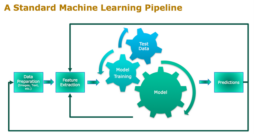
Diagrammatic Approach of End-to-End Machine Learning Modelling. Image Credits: Datanami
It allows us to directly take an input X to make a prediction Y, without needing to go through any intermediate process in the midst. Developing an End-to-End Machine Learning Model allows us to create scalable models that can be served to multiple users and allows real-time processing.
In traditional Machine Learning, the historical data is collected, pre-processed, modelled using a specific algorithm, and then compared for the Scores. In comparison, an End-to-End Machine Learning Model prefers to collect the data, stream it for features, and use the existing models to generate some results. In this project, we will be developing a Machine Learning Pipeline, which can be directly served to an application and check if a message is “Spam” or “Ham.”
Data Collection and Exploratory Data Analysis
We will be using the SMS Spam Collection Data Set from UCI Machine Learning Repository, a collection of 5574 Text Messages for Classification and Clustering purposes. The messages are suitably labelled “Spam” or “Ham,” and we can use it to model our Machine Learning Model.
Let’s first load our Dataset using Pandas Library that is a popular library used for generating Dataframes and preparing the Data for final modelling.
import numpy as np
import pandas as pd
messages = pd.read_csv('SMSSpamCollection', sep='\t',names=["label", "message"])
We have divided our Dataset into two columns: labels and messages. The label denotes whether the message is “Spam” or “Ham,” while the message is the actual message for which the label has been kept. Once we have loaded our Dataset, we can move forward with some Exploratory Data Analysis to better analyze our Dataset and move forward with the final implementation.
Let’s do some Exploratory Data Analysis before we move forward with our final implementation. We can check out some of the parameters in our Data using Pandas. Let’s check out the length of the text:
import matplotlib.pyplot as plt
import seaborn as sns
%matplotlib inline
messages['length'] = messages['message'].apply(len)
messages['length'].plot.hist(bins=100,histtype='bar',ec='black')
This is what we get as the output:

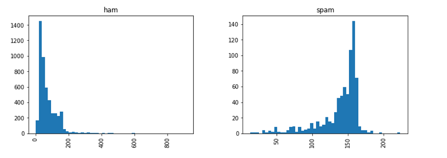
Let’s go forward and check out the length of “Spam” and “Ham” messages each:
messages.hist(column='length',
              by='label',
              bins=50,
              figsize=(12,4))
In the below graph, we can see that the message's length is an essential parameter to judge whether a message is spam or not. Here we can see that Spam messages tend to have more characters compared to Ham messages:
So we have sorted out our Feature Engineering, so we can move forward with pre-processing our Dataset and fine-tuning it for our Data Modelling.
Dataset Pre-Processing
In this Dataset, all the input variables are in the form of Strings. Machine Learning Algorithms, on the other hand, tend to use numerical vectors to model the data and generate predictions. In this case, we will be converting our whole Dataset into a numerical value that can be processed by our Machine Learning Model quickly.
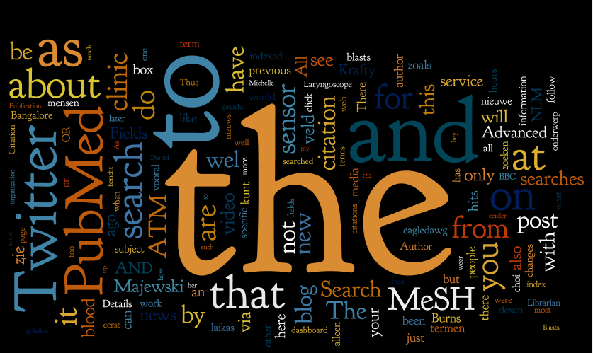
Stopwords in English. Credits: XPO6
To make this possible, the raw messages, which are a sequence of characters, are converted into a sequence of numbers, and for this, we will use the Bag-of-Words approach where all the characters are denoted by one digit. To make this possible, we will first go through removing Stopwords from our strings. Stopwords are used by people in general and do not hold any significance in Data Modelling Operations.
Let us define a function that can take in any string and remove the Stopwords and Punctuations from it. We will be using the NLTK library for the same to remove the stopwords for this purpose.
def text_process(mess):
    nopunc = [char for char in mess if char not in string.punctuation]
    nopunc = ''.join(nopunc)
    return [word for word in nopunc.split() if word.lower() not in stopwords.words('english')]
Now that we have removed the Stopwords and Punctuation from the Dataset, we can normalize the Dataset. We will now be converting all the words in the Dataset to a form that can be operated on by Scikit-Learn Machine Learning libraries.
We will be doing this in the form of three well-defined steps: First, we will calculate the term frequency, which denotes the number of times a word occurs in a dataset. Next, we will weigh the counts so that the frequent tokens get the lower weigh, which is called the inverse document frequency. We will convert the vectors to unit length to abstract from the original text length, namely the L2 Norm.
Let’s use Scikit-Learn’s CountVectorizer to convert the Dataset into a sparse matrix and visualize how we have transformed the String into a Vector:
import string
from nltk.corpus import stopwords
from sklearn.feature_extraction.text import CountVectorizer
bow_transformer = CountVectorizer(analyzer=text_process).fit(messages['message'])
messages_bow = bow_transformer.transform(messages['message'])
We have used the transform() function the entire Dataframe of the messages into a large, sparse matrix. We can now use another methodology named TFIDF or term frequency-inverse document frequency to check and highlight any word's importance in a collection of the corpus. So, let's go ahead and implement this with our Dataset:
from sklearn.feature_extraction.text import TfidfTransformer
tfidf_transformer = TfidfTransformer().fit(messages_bow)
messages_tfidf = tfidf_transformer.transform(messages_bow)
We have now normalized our whole Dataset, and we can finally move forward with our Data Modelling. We will also be building a pipeline to serve our Model, yet which is our article's final purpose.
Data Modelling
For Data Modelling, we will be using a Naive Bayes classifier. We are using the Naive Bayes Classifier because it is quite simplistic, and it helps us achieve results that outperform many complex algorithms, especially in Classification Problems. Here we can use the Naive Bayes classifier for our purpose by developing a distribution over words to simplify our task.
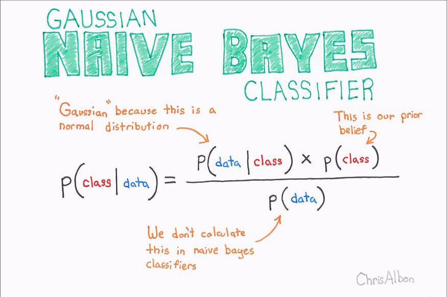
Credits: becominghuman.ai
We will implement the Naive Bayes using the Scikit-Learn implementation for the same, which will help us write minimal code for the task at hand:
from sklearn.naive_bayes import MultinomialNB
spam_detect_model = MultinomialNB().fit(messages_tfidf, messages['label'])

# Let's check out the output
message4 = messages['message'][3]
bow4 = bow_transformer.transform([message4])
tfidf_transformer = TfidfTransformer().fit(messages_bow)
tfidf4 = tfidf_transformer.transform(bow4)
print('predicted:', spam_detect_model.predict(tfidf4)[0])
print('expected:', messages.label[3])

'''
>> predicted: ham
>> expected: ham
'''
Pretty easy with that? We modelled our Pre-Processed and clean Dataset in just two lines of code! Let us now evaluate our model's performance that we have developed using yet another Scikit-Learn’s Library: classification_report.
from sklearn.metrics import classification_report

all_predictions = spam_detect_model.predict(messages_tfidf)
print (classification_report(messages['label'], all_predictions))

'''
precision    recall  f1-score   support

        ham       0.98      1.00      0.99      4825
       spam       1.00      0.85      0.92       747

avg / total       0.98      0.98      0.98      5572

'''
We can now check out the Classification Report for the model that we have prepared. However, we have just evaluated on the same dataset that we have only trained the model on. We will now follow another methodology to test our model by dividing (or splitting) the dataset into two parts: Train and Test.
Let’s use another Scikit-Learn Library, known as train_test_split, to split our dataset into two parts. We can use 20% of the dataset for testing, while the rest 80% can be used for training the dataset.
from sklearn.model_selection import train_test_split

msg_train, msg_test, label_train, label_test = train_test_split(messages['message'], messages['label'], test_size=0.2)

print(len(msg_train), len(msg_test), len(msg_train) + len(msg_test))
Preparing the Pipeline
Let us now arrive at the central part: Preparing our Pipeline to serve our Model. We have loaded the Dataset, pre-processed, and cleaned the Dataset in the previous steps, but now we need to move ahead with creating a Pipeline. A pipeline will help us automate all our workflow in one single step and a few lines of code, so let’s try it out.
We will be leveraging the Scikit-Learn’s Pipeline library to model our Dataset and develop a pipeline. This can be treated as an Application Programming Interface (API), which can be directly served to some Web Application, allowing us to perform the computations real quick.
from sklearn.pipeline import Pipeline

pipeline = Pipeline([
    ('bow', CountVectorizer(analyzer=text_process)),
    ('tfidf', TfidfTransformer()),
    ('classifier', MultinomialNB()),
])

pipeline.fit(msg_train,label_train)

predictions = pipeline.predict(msg_test)

print(classification_report(predictions,label_test))


'''

             precision    recall  f1-score   support

        ham       1.00      0.95      0.98      1003
       spam       0.71      1.00      0.83       112

avg / total       0.97      0.96      0.96      1115
'''
In a few easy steps, we have now set our Pipeline Model, which can now be served with an API, to some Client-Side Interface, and we don’t need to take care of all that background processes anymore.
Conclusion
In this article, we have covered many aspects of why Pipelines are needed to serve End-to-End Machine Learning Models and how we can classify “Spam” or “Ham” messages using a Naive Bayes Algorithm. Naive Bayes works so well because it works on the assumption that the features of the dataset are independent of each other.
We have also got to know how we can serve the Model using a Pipeline, and in further articles, we will get to see how we can directly serve it using a Flask API on a Client-Side Interface while learning the basics of Flask on the way.
Check out the Code here.

